Learning How to Learn Where You Are: Meta-Learning for Few-Shot Camera Localization using AWS

Dominik Kloepher – AIMS CDT Student

Problem Setting

In this project, we looked at the task of camera localization: given a number of images of a scene (a room, a street, …) and the positions and viewing directions from which they were taken (together, these are the camera pose), can we determine the camera pose from which a new, unseen image was taken?

A method that could do so reliably and quickly would find use in many different fields, from robotics and autonomous driving (to determine where to go, the self-driving car needs to know where it is!) to augmented reality applications (to determine what virtual objects to overlay at what point in the scene, the AR-device needs to know where it is itself).

Given how widely applicable camera localization is, it is no surprise that many different methods have been proposed to solve this problem. Some aim to use correspondences between distinctive features in the image and these features in some internal 3D-representation of the scene to then triangulate the camera pose, while others train neural networks to directly predict the camera pose from an image directly.

These methods however have some significant drawbacks: The former class of methods usually requires a detailed 3D-scan of the scene to establish these correspondences between image and the 3D-structure of the real world, and these scans are time-consuming and expensive to collect. The neural-network-based methods on the other hand usually require many (several thousand) images to learn a single scene, and need to be re-trained from scratch for each new scene. Neural-network-based systems also usually do not perform as well as the 3d-structure-based methods achieve on most camera-localization benchmarks.

Method

DSAC

To address these challenges, we built our method based on a previous method, DSAC [1], which achieved state-of-the-art results on several camera localization datasets.

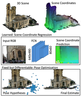
DSAC in a way is a hybrid of the 3D-structure-based and the neural-network-based methods. It uses a neural network to predict the 3D-world-coordinates of the pixels in the image to establish the correspondence between the image and the real world, and then uses these correspondences to triangulate the camera pose. Establishing these image-to-world correspondences using a neural network means that DSAC does not require a detailed point cloud, while its use of triangulation still allows it to perform very well.

Intuitively, the neural network picks out some distinctive landmarks (e.g. a chair) in the scene and memorises their 3D real-world coordinates. If it then sees some of these landmarks in a test image, it can solve the question “if this chair appears in the left part of the image, and I know that it is at this position in the scene, where must I (the camera) be for the chair to appear where it does?” to determine the camera pose. This is visualised in Fig. 1.

Fig. 1: Visualisation of the method of DSAC. Image taken from [1].

Meta-Learning and Our Method

Despite its advantages, DSAC still requires a large number (at least 1000) images to learn to localise a camera in even small scenes. Inspired by previous research on few-shot-learning (that is, machine learning based on only very small datasets), we decided to extend DSAC with meta-learning techniques. The field of meta-learning generally aims to use a network’s experience on many related, but different, tasks to enable it to learn how to perform well on a new task more quickly. This is often described with the phrase “learning how to learn”.

Following the technique described in [2], we split the network that predicts the world-coordinates of pixels in two: One part, the feature extractor stays fixed for a single scene, while the second part, a simple linear regression, is adjusted for each new scene (this can be done efficiently simply by computing the closed-form solution). The weights of the feature extractor are then adjusted after each scene so that the linear regression will do better at predicting the 3D world-coordinates of pixels.

The idea behind this is that the feature extractor will learn to recognise parts of scenes that would be god landmarks, making it easy for the linear regression to remember the 3D-world coordinates of these landmarks.

Because for each scene only a small number of weights is adjusted, fewer datapoints (i.e., fewer images of the scene) are required to memorise a scene. Due to the simplicity of the linear layer, overfitting of the network is also unlikely to be a problem.

Fig. 2 shows a diagram of our method.

Fig. 2: Diagram of our method, which extends DSAC [1] using the meta-learning technique from [2]. The meta-trained feature extractor embeds a test image to make it easier for the linear layer to predict the scene coordinates. Using a Perspective-n-Pose algorithm in a RANSAC loop, the camera pose is then triangulated.

Training using AWS

Our method has one drawback: the training of the linear layer requires all the images from one scene to be loaded into the computer’s memory at the same time. Even though we reduce the number of images required for each scene by a factor of more than 10, the memory required still exceeds that available to most GPUs. Even when distributing the training across multiple GPUs, the memory requirements remained substantial.

Here, access to cloud services from Amazon Web Services (AWS) was very valuable. The Elastic Compute Cloud (EC2) service allowed us to select the instance type with the necessary GPU capacity, which in this case was the g4dn.12xlarge instance. To safeguard against possible crashes and to be able to straightforwardly continue training after terminating the instance for a short period, we added 64GB of Elastic Block Storage (EBS) to that instance.

The g4dn.12xlarge instance gave us access to 4 high-end GPUs with 16GB of memory each for 64GB of GPU memory in total. Even when ignoring the benefit of increased GPU memory, using higher-end and more powerful GPUs on its own increased training speed, even when increasing the batch size. On the departmental server, jobs would usually run for six days to a week, while we achieved a similar number of training steps in roughly four-and-a-half days on the AWS instance, and that while using more GPU memory.

Citations

[1] Eric Brachmann and Carsten Rother. Learning less is more - 6d camera localization via 3d surface regression. In 2018 IEEE/CVF Conference on Computer Vision and Pattern Recognition, pages 4654– 4662, 2018

[2] Luca Bertinetto, João F. Henriques, Philip Torr, and Andrea Vedaldi. Meta-learning with differentiable closed-form solvers. In International Conference on Learning Representations, 2019.